compare Search Operator
The compare operator can be used with the Time Compare button in the Sumo interface, which automatically generates the appropriate syntax and adds it to your aggregate query. The following information can also be found documented in Time Compare.
You can use compare to:
- Evaluate the performance metrics of a website, such as the latency or the number of exceptions, before and after a deployment.
- Track the root cause of a production issue quickly by tracking specific keywords, such as memory exceptions, and comparing them with historic data to find any anomalous trends.
- Compare the daily active or weekly active users on your website for strategic business insights.
- Identify malicious activity or attacks by comparing failed login attempts against past averages.
Use the compare operator in the following ways:
- Compare with a single time period in the past.
- Compare with multiple time periods in the past.
- Compare with an aggregate over multiple time periods in the past.
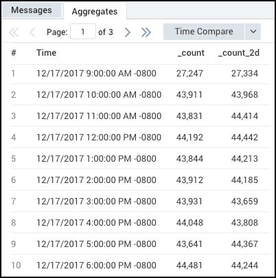
By default, results are displayed in the Aggregates tab on the search page in a table. Each column of the output table contains results from one of the specified queries. The first column is suffixed with the keyword target, appended to the original column name, and contains results from the present time (or the time range specified in the time range field). Additional columns are suffixed by the timeshift (the period shifted back in time) of the queries. From here, you can select a chart type to display results visually.
For example, if you were doing a comparison with yesterday, when you use the compare operator after the count operator, the aggregation table results will display the column names count_target and count_1d.
Syntax
Single Comparison
Compare the present results with a single time period in the past. To make the comparison, specify the time interval you want to go back, in the form of number and time granularity:
... | compare timeshift <number><time granularity>
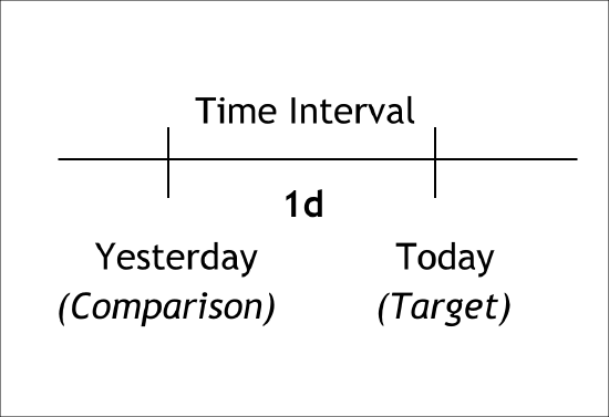
The following query returns data from the present, along with results from yesterday. Here the parameter 1d specifies the time interval we want to go back to get the data for the comparison.
... | compare timeshift 1d
This comparison can be displayed visually as:
In another example, this query returns data from the present along with results from last week.
... | compare timeshift 1w
Multiple Comparison
Compare the present results with multiple time periods in the past. The first parameter specifies the time interval between the present query and the most recent comparison point. The second parameter specifies how many comparison points to create.
... | compare timeshift <number><time granularity> <number of timeshifts>
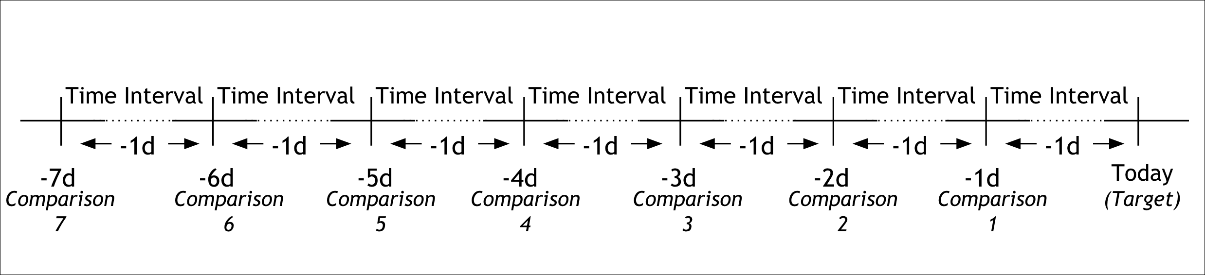
The following query returns results from the present, along with results from every day of the past week. The first parameter, 1d, specifies the interval between the points of comparison, and the second parameter, 7, specifies the number of comparisons.
... | compare timeshift 1d 7
Which can be displayed visually as:
The following query returns result from the present with results from the same day in the last 3 weeks. So if today is Monday, then this query will show a result for today and the last three Mondays.
... | compare timeshift 1w 3
Aggregate Comparison
Aggregate the results from multiple past time periods using an aggregation operator (avg, min, or max).
... | compare timeshift <number><time granularity> <number of shifts <avg/min/max>
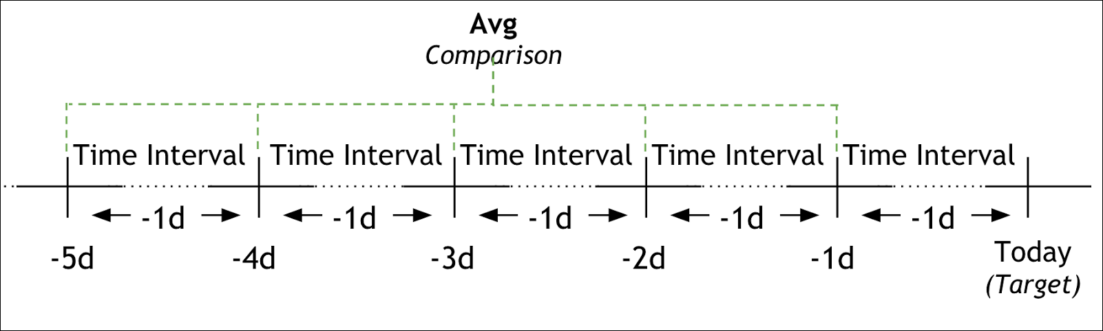
The following query returns results from the present along with the average of the results from the last five days:
... | compare timeshift 1d 5 avg
Which can be displayed visually as:
Other examples:
- Maximum of the same day for last three weeks:
... | compare timeshift 1w 3 max - Minimum of the last four six-hour intervals:
... | compare timeshift 6h 4 min
Advanced
You can also do multiple different comparisons queries under the same compare operator by using multiple timeshift phrases separated by commas.
... | compare\<comparison >,\<comparison >, ...
For example:
... | compare timeshift 12h, timeshift 1d 3 avg, timeshift 1w
You can specify an alias, and the columns generated use the name you specify.
... | compare <comparison 1>, <comparison 2>, ...
For example:
... | compare timeshift 1d as yesterday, timeshift 1w 4 as last_four_weeks
Rules
- The compare operator must follow a group by aggregate operator, such as:
count,min,max, orsum. - If you want to use
timeslicewithcompare, do not aliastimeslice.
Limitations
-
Compare cannot generate more than seven additional queries. An additional query is generated whenever a comparison in time is initiated. Note that multiple comparisons and aggregate comparisons will generate multiple queries. For example, the following queries are not allowed:
... | compare timeshift 1d 14This query compares with the past 14 days data. It is not allowed as it generates 14 queries.
... | compare timeshift 1d 5 avg, timeshift 1w 4This query compares with the last five days, and the same day for the last four weeks. It is not allowed as it generates 9 queries.
-
Duplicate aliases are not allowed. For example, the following query is not allowed:
... | compare timeshift 1d 7 as last_week, timeshift 1d 7 avg as last_week -
Real-time queries using time compare need to have at least three timeslices within its time range. For example, if the time range is 10 minutes, your timeslices need to be no longer than 3 minutes so that there are at least three of them.
-
Compare is not supported in Scheduled Views.
-
Compare can only be used once in a search query.
Examples
Compare time series data with past data
Use compare to analyze the change in log counts between two days.
error
| timeslice by 1h
| count by _timeslice
| compare timeshift 2d
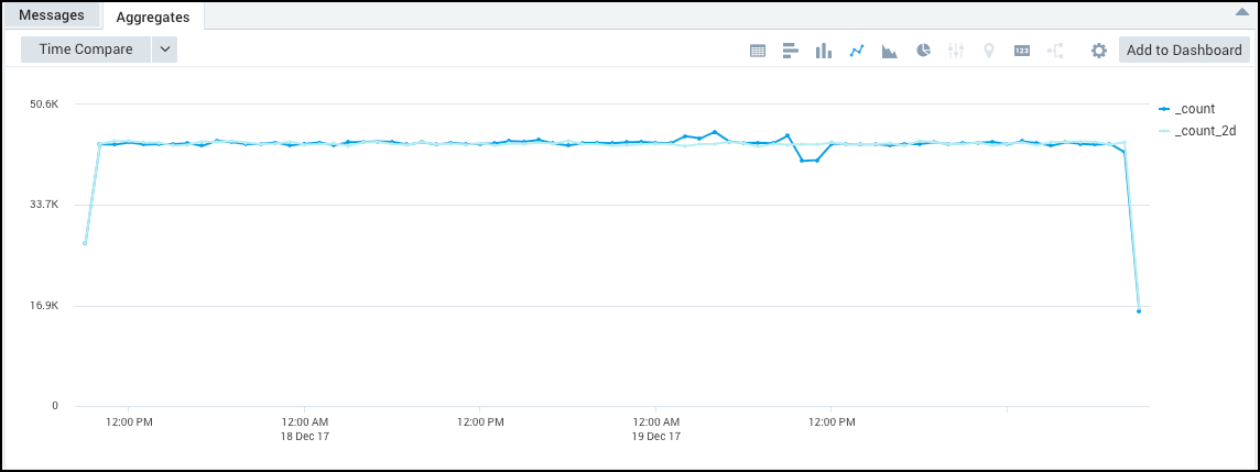
The query returns results from both today and two days ago, with each day in its separate column. Today's results are represented by _count.
Create a line chart to visualize the results.
Using the multiple comparison feature, you can compare the number of logs against every ten minutes of the past hour:
_sourceHost = prod
| timeslice by 1m
| count by _timeslice
| compare timeshift 10m 5
Each ten-minute period produces its own column in the output table:
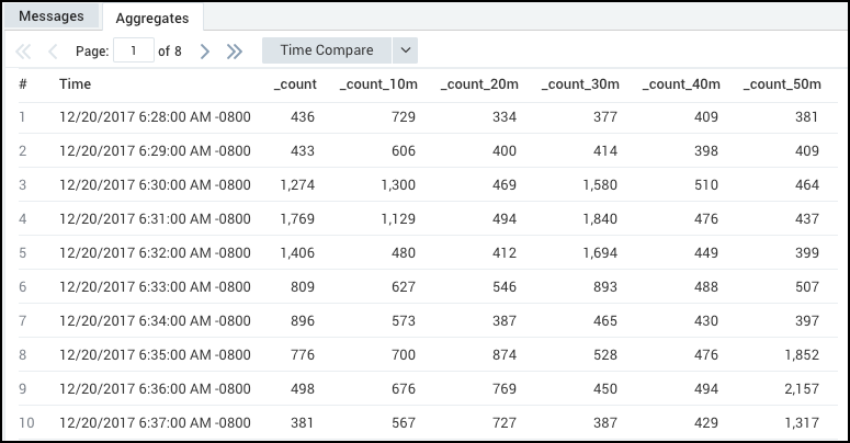
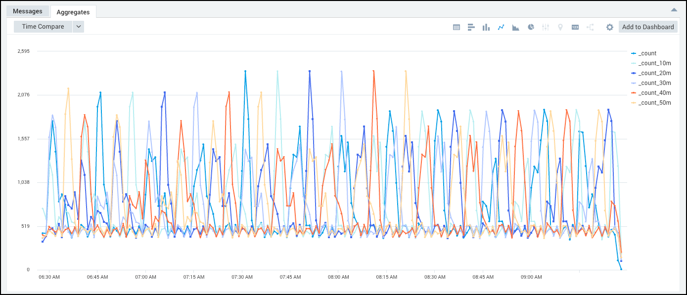
Create a line chart to visualize the results.
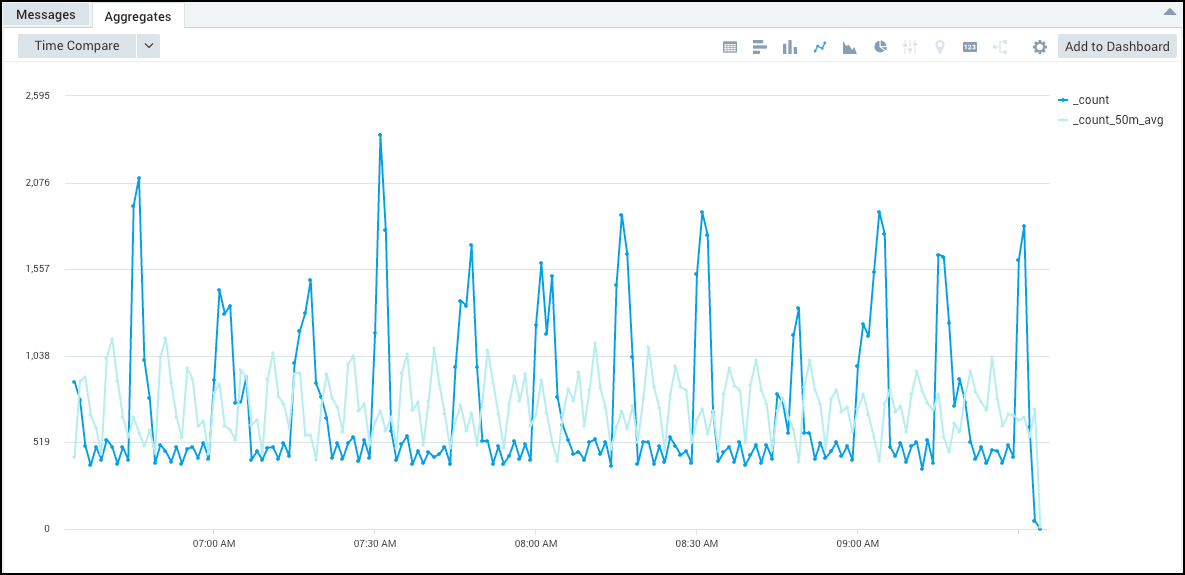
Alternatively, you can compare against the average of all the ten minute periods:
_sourceHost = prod
| timeslice by 1m
| count by _timeslice
| compare timeshift 10m 5 avg
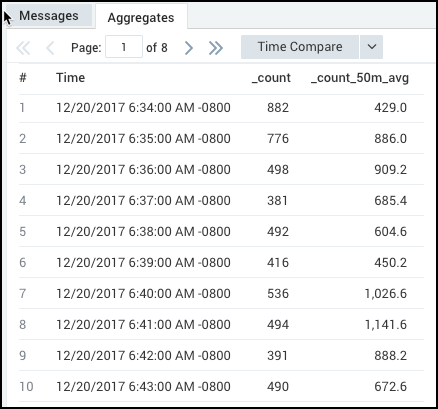
Create a line chart to visualize the results.
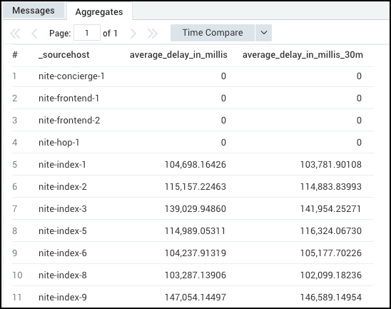
Compare categorical data parsed from logs
Use compare to analyze the change in delays on different _sourceHosts using parsed data from logs.
"delay:"
| parse "delay: *" as delay
| avg(delay) as average_delay_in_millis by _sourceHost
| compare timeshift 30m
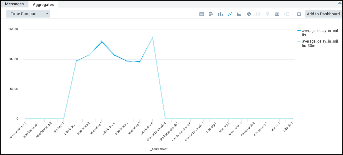
This example computes the average delay per _sourceHost, and compares with results from 30 minutes ago.
These results would create a line chart such as the following.
Compare after a Transpose operation
You can use the compare operator after a transpose operation, such as the following:
_sourceCategory=analytics
| timeslice 1m
| count by _timeslice, _sourceHost
| transpose row _timeslice column _sourceHost as %"nite-analytics-1", %"nite-analytics-2"
| compare with timeshift 15m